you come across a functional form in a paper or online which you think might be useful.. a distribution, a gain curve, a something.. you find a formula, see a few plots, and decide, sure, that might work..

now, translating a formula from a paper into some sort of code shouldn't be an issue, it's not a difficult thing to do.. and yet, it's something I've gotten wrong on more than a few occasions.. and the longer it takes to find your mistake the more annoying this mistake is sure to become..

anyway, the problem.. you want to reproduce a plot you've seen, with a given formula.. one of the simplest ways in my book to do this is to overlay your plot on the one you're looking at.. this isn't particularly difficult to do, but it's one of those things that (at least for me) always takes longer than it should

a worked example

here we have an excerpt from wiki's article on the gaussian function which includes the formula and a plot..

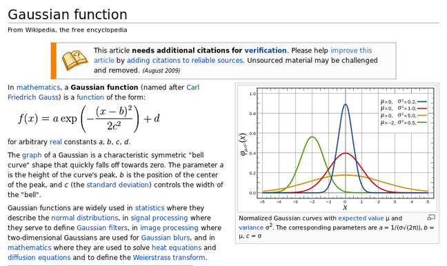
the first thing to do is to get the highest possible res version of the plot, most pdf readers allow you to take snapshots for this.. or in the case of this wiki article, we can just get a decent resolution image pretty easily

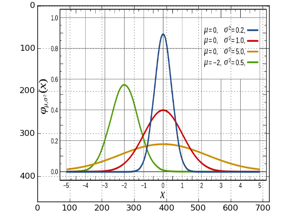
1. importing the image..

from pylab import *

img = mpl.image.imread('gaussian_figure_from_wiki.png')
imshow(img, aspect='auto')
grid(True)

the aspect='auto' preserves the aspect ratio of the image.. but the matplotlib axes are in terms of pixels, which, seems to be standard for imaging work, though not being particularly useful for our purposes..

2. reconciling coordinate systems

reconciling the matplotlib coordinate system with the coordinates of our chosen plot isn't difficult either, but requires a bit of messing around.. it's done with the extent argument, which we pass to imshow.. in order to do it correctly, we need to scale and shift our image, so that the axes match..

from pylab import *

#put the initial guesses in the 'extent' argument, here I've taken -5,5 and 0,1

#start off with _shift and _scale y as 0 and 1./1.
#then, line up the 0's with _shift, before finally messing with the scaling
#until everything lines up

x_shift = 0.4
x_scale = 1./.835

y_shift = 0.15
y_scale = 1./.79

extent = [ x_scale*(-5. - x_shift), x_scale*(5. - x_shift),  y_scale*(0. - y_shift ), y_scale*( 1. - y_shift)]

img = mpl.image.imread('gaussian_figure_from_wiki.png')
imshow(img, aspect='auto',extent=extent)
grid(True)

all going well, this will leave us with..

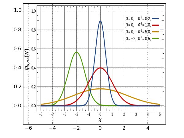
you can see here that the gridlines don't match up exactly, but as far as I'm concerned...

3. doing other stuff...

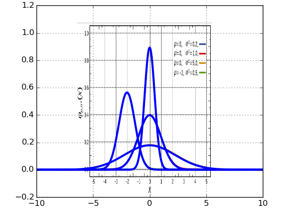
now we're pretty much done with the heavy lifting (not that heavy in fairness)... but if, for example we wanted to see what the gaussian (or more likely, some other more exciting function) looked like outside the range of the plot we're given.. we can do..

from pylab import *

def gaussian( a, b, c, d, x ):
  return a*exp( -  ((x-b)**2.)/( 2*(c**2.))) + d

x_shift = 0.4
x_scale = 1./.835

y_shift = 0.15
y_scale = 1./.79

extent = [ x_scale*(-5. - x_shift), x_scale*(5. - x_shift),  y_scale*(0. - y_shift ), y_scale*( 1. - y_shift)]

img = mpl.image.imread('gaussian_figure_from_wiki.png')
imshow(img, aspect='auto',extent=extent)

x = arange(-10, 10, 0.01)

for mu, root_sigma in zip([0,0,0,-2], [0.2, 1.0, 5.0, 0.5]):
  sigma = root_sigma**0.5
  a = 1./(sigma * (2*pi)**0.5 )

  plot( x, gaussian(a, mu, sigma, 0, x), 'b', lw=3)
grid(True)